The discussion at the clean-water plant operators’ meeting was the same as before: How will we prevent fecal coliform excursions this season? It seems to be a common topic at these meetings and normally comes up right before the change from summer to fall and spring to summer.

What could be causing the frequent out-of-compliance issues that only seem to occur in April and May, or October through November? The plant’s managers were weary of having to sit in county commission meetings and explain why the state had levied fines on the facility for noncompliance with permitted fecal coliform discharge limits.

The Lab Detective was on a training mission in a nearby county when he was asked to attend a meeting of operators and managers at a plant that was having problems meeting coliform limits. Always one to oblige, he arranged to be at the meeting.

Gathering data

The meeting between operating staff, laboratory personnel, plant managers and engineers was very interesting. The group tossed around many ideas about what to do in the coming season to maintain compliance and avoid costly fines and negative publicity. The detective gathered as much data as he could while listening to the banter across the conference room table. The data he gathered during the discussion:

• The facility is designed for 20 mgd.
• The average daily flow rate during the excursions is 12 mgd.
• The plant is a complete-mix activated sludge facility, using diffused aeration.
• There are no nitrogen or phosphorus limits in the discharge permit.
• The plant is required to monitor and report value for effluent total nitrogen.
• Effluent permit limits for CBOD and TSS are 30 mg/L annual average.
• Limits for fecal coliform are 200 cfu/100 mL annual average, 500 cfu/100 mL weekly average, 800 cfu/100 mL daily maximum.
• The plant uses anaerobic digesters for biosolids stabilization.
• The plant dewaters biosolids on site; cake is trucked to landfill.
• The facility switched disinfection to sodium hypochlorite (12 percent solution) from gas chlorine several years ago.
• The facility had no coliform excursions when using gas chlorine.

Using the information from the meeting, the detective returned to his office to put the pieces of the puzzle together. Thinking back to the meeting, he recalled a question the operators asked the lab personnel: Where on the breakpoint curve are we?

The chlorine residual breakpoint curve

The breakpoint curve for residual chlorine is familiar to most all drinking water treatment plant operators, but not necessarily to wastewater operators. This is because most utilities that are required to provide chlorination disinfection to their public drinking water supply measure the residual as “free” chlorine residual. Providing free chlorine residual helps protect the public water supply from bacterial contaminants by maintaining a strong acid that can kill most pathogenic organisms.

Clean-water plant operators are normally required to maintain what is known as “total” chlorine residual, which may contain some free chlorine acid or not. One of the key factors in the kind of residual present in plant effluent is the amount of ammonia available. Let’s look at what happens when chlorine, water and ammonia get together.

When the plant described above used gas chlorine, the disinfection chemistry was pretty straightforward. Gaseous chlorine is very soluble in water. Most all gas chlorinator units have a water feed that provides a vacuum when the water is forced through a venturi in the chlorine ejector. The vacuum sucks the gas chlorine from the bottle and allows it to dissolve rapidly in the feedwater, quickly forming hypochlorous (HOCl) and hydrochloric (HCl) acids.

Of the two acids, the more powerful is the HOCl. HCl falls apart rapidly in the presence of water and forms H3O (hydronium) and Cl (chloride). The HOCl is thought to contain a nascent oxygen atom that is the actual oxidizer (killer) of bacteria. Once the strong chlorine solution is formed after the ejector, the solution can be applied to the plant effluent.

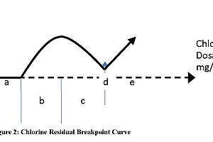
Before any chlorine residual is seen, the applied chlorine reacts with any reducing agents that might be present in the effluent: organic material, dissolved iron or manganese, hydrogen sulfide and nitrite. Chlorine is very reactive: It readily oxidizes these reducing agents, and there is no residual seen at all (Figure 1). This is called chlorine demand, and it makes up the initial stage of the breakpoint chlorine curve (Figure 2, letter a).

Ammonia interaction

After the chlorine demand has been met, the available chlorine begins reacting with any ammonia present. Most wastewater plants have ammonia entering with the influent wastewater, and some plants biologically remove or convert the ammonia as part of the treatment process. Treatment plants that use anaerobic digestion, including the facility described here, normally return supernatant from the secondary digester to the head of the plant, and this supernatant contains high amounts of ammonia.

Chlorine and ammonia bond together and make new compounds called chloramines. The amount of chloramine and what type of chloramine depends on several factors; the amount of chlorine and ammonia, pH and temperature of the water are just a few.

There are three types of chloramine: monochloramine, dichloramine and nitrogen tri-chloride (trichloramine). As chlorine is fed into the water that contains ammonia, monochloramine is formed first, and dichloramine forms as chlorine dosage increases. Trichloramine is not generally formed until the water pH drops significantly, to less than about pH 5.

Monochloramine and dichloramine do have disinfecting capability but not as strong as HOCl. For HOCl to become present, we need to feed enough chlorine to overcome (oxidize) the chloramines that were produced. On the breakpoint chlorine residual curve in Figure 2, we would now be in the “curve part” between b and c. If we measure chlorine residual using the total chlorine DPD reagent, we would now get a pink color, indicating that chlorine residual is present. If we use the DPD free chlorine reagent, we would still not see a pink color develop, since we have not yet reached the “breakpoint.”

As monochloramine and then dichloramine increase with a rising chlorine feed, we reach the “hump” of the curve. At a certain ratio of chlorine and ammonia, the amount of chloramine starts to decrease, since the chlorine is destroying (oxidizing) the dichloramine and monochloramine previously formed. The total chlorine residual using the DPD reagent would now be decreasing.

Dichloramine decomposes first, then monochloramine. We get to a certain point where the residual bottoms out, still giving a pink color with the DPD reagent, but a very low residual amount. You’ll notice on the breakpoint curve in Figure 2, letter c, that the residual line does not actually reach zero before hitting the breakpoint at letter d. This area is where chlorine residual might be found using the DPD residual reagent, but is not actually true chlorine residual. Any chlorine that interacted with organic material present in the water forms chloro-organic compounds, which interfere with the DPD reagent and create a pink color — a false residual value, sometimes called “nuisance residual.”

Affect of pH

As chlorine dosage continues to increase, we enter the zone after the theoretical breakpoint (Figure 2, letter d) where free chlorine residual is now seen with the DPD free chlorine residual reagent. For every milligram of chlorine dosed per liter, we get an equal amount of free chlorine residual, mg/L (letter e, Figure 2).

The liquid’s pH value influences the type of chloramine present, as well as how much HOCl is produced. When effluent pH values are near 7.0, monochloramine and dichloramine can exist together. The dichloramine tends to be the stronger of the two and favors lower pH values, while monochloramine favors higher pH values.

The facility in this situation had switched from gaseous chlorine to sodium hypochlorite (strong bleach solution) and began experiencing problems certain times of the year. Sodium hypochlorite is usually about 12 to 15 percent available chlorine and is produced commercially for the water and wastewater industry. We find that the use of sodium hypochlorite tends to raise the pH of the liquid it is applied to; the sodium component is a high alkali metallic material.

As pH values rise, the amount of available HOCl produced at the ejector decreases, and the amount of hypochlorite ion (OCl-) increases. The HOCl is the stronger of the two and is the chlorine species we like to have present for killing bacteria. The higher the pH, the lower the amount of HOCl, and the higher the OCl-.

At pH 7, about 78 percent of the available chlorine is in the form of HOCl, and about 22 percent OCl-. At pH 8, just one pH unit higher, the available HOCl drops to about 22 percent, and the OCl- climbs to 78 percent, essentially trading percentage places.

Think of the HOCl as shooting the pathogens with a .44 caliber bullet — one shot and it’s dead! Think of the OCl- as a .22 caliber bullet. It might take many more hits with the .22 to effectively kill the coliform bacteria. All bacteria have an external slime coating, or layer, that must be penetrated by the disinfectant to effectively kill the cell.

HOCl is a neutrally charged chemical (neither positive nor negative). OCl- is negatively charged, as is the slime layer of the coliform bacteria, so they tend to repel each other like the negative poles of two magnets. It takes more of the OCl- disinfectant and longer contact time to get the required inactivation of the coliform bacteria.

Finding answers

This is essentially where the facility was with its disinfection problem. The facility regularly had an effluent pH value of 8.0 to 8.2 since using sodium hypochlorite solution as the disinfectant. The effluent pH normally had been about 7.0 when using gaseous chlorine. The Lab Detective returned to the facility with the information he had found. In a meeting with the operators, he offered some options to resolve the problem.

First, ensure adequate contact time in the chlorine contact basin. Even in the monochloramine residual zone, coliform destruction can still occur with enough contact time. Second, ensure that the contact tank is clean and free of settled solids, even algae. Chlorine will react and oxidize solids, which create chlorine demand. Suspended solids can also provide a protective barrier for pathogens to hide from the disinfectant. Third, always ensure good mixing of the chemical with the water being treated.

During problem times of the year, feed more bleach, essentially raising the dosage of available chlorine. Feed some acid along with the bleach to maintain a pH of about 7.0 to 7.2. Try to stay in the dichloramine zone, near the “hump” of the curve, if electing to avoid reaching breakpoint.

Use caution when supernating the anaerobic digesters and avoid supernating during the peak flows of the day. The Lab Detective recommended returning this supernatant during times of low flow and returning this liquid slowly to avoid organic and hydraulic overload. Remember, the ammonia content in the supernatant will affect the amount and type of chloramine produced.

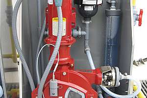
As this article was written, the facility staff reported to the Lab Detective that they had so far been in compliance by maintaining a slightly reduced pH. They did this by adding some sulfuric acid to the inlet of the contact tank and thoroughly cleaning the contact tank and hypochlorite feed pump discharge tubing and lines. They also checked the hypochlorite feed pump discharge flow rate using the pump system drawdown tubes to verify the actual flow from the pumps (Figure 3). By also following the anaerobic digester supernating recommendation, the facility can now maintain aeration tank dissolved oxygen much more effectively.

About the author

Ron Trygar is senior training specialist in water and wastewater at the University of Florida TREEO Center and a certified environmental trainer (CET). He can be reached at rtrygar@treeo.ufl.edu.

References
[1] “Chemistry of Water Treatment,” Second Edition; Samuel Faust and Osman Aly; 1998 CRC Press LLC.
[2] “Water Chlorination/Chloramination Practices and Principles, M20,” Second Edition, 2006 AWWA.